Agent skills for researchers

Skills that automate
the academic grind.

I'm a PhD researcher. I build agent skills for the parts of research that eat the week: digging through literature, wrangling data, making figures, and getting drafts into shape. The skills live on Agensi. This page shows what they produce.

  • Literature
  • Data analysis
  • Scientific visualization
  • Writing & polishing

Sample outputs

One toy topic, start to finish

Every example below works on the same small problem, the logistic map xn+1 = r xn(1 − xn), so you can follow it from reading list to finished paragraph. Numbers are computed, citations are real, and every figure is reproducible from src/figures.py.

  1. 01Literature brief
  2. 02Analysis
  3. 03Figures
  4. 04Polished prose

01 · Literature

A reading brief, not a pile of PDFs

You ask"Give me the essential papers on why the logistic map goes chaotic, and how they fit together."

You get a short brief: the question, the few papers that matter, one line on why each one matters, how they connect, and where to read next.

Reading brief

Why does a one-line model go chaotic, and what is universal about it?

  1. Sharkovskii (1964), Coexistence of cycles of a continuous map of the line into itself. Ukrainian Mathematical Journal 16, 61–71. Orders the integers so that a continuous interval map with a cycle of period m must have cycles of every period that comes after m. Period 3 sits at the top: it forces all the others.
  2. Li & Yorke (1975), Period three implies chaos. The American Mathematical Monthly 82(10), 985–992. Independently shows that period 3 forces every period, plus an uncountable set of non-periodic orbits. This is where "chaos" got its mathematical name.
  3. May (1976), Simple mathematical models with very complicated dynamics. Nature 261, 459–467. Brings the logistic map to a wide audience, walks through the period-doubling route, and argues it should be taught early.
  4. Feigenbaum (1978), Quantitative universality for a class of nonlinear transformations. Journal of Statistical Physics 19(1), 25–52. The gaps between successive period doublings shrink by a universal factor δ ≈ 4.6692, the same for any smooth map with a quadratic maximum.

How they connect

Sharkovskii and Li–Yorke say which periods must coexist. May shows the route a real model takes. Feigenbaum explains why that route looks the same across models.

Read next

Lanford (1982), A computer-assisted proof of the Feigenbaum conjectures, Bulletin of the AMS 6(3), 427–434: the step from numerical observation to proof. Open thread: δ depends on the order of the map's maximum, so a non-quadratic peak lands in a different universality class.
02 · Data analysis

Numbers with the method and the caveats attached

You ask"Estimate Feigenbaum's δ numerically and tell me how much to trust it."

You get the result, the table behind it, how it was computed, and what limits the precision, so it can go straight into a methods section.

Analysis note

Estimating δ from superstable parameters

Result. δ ≈ 4.669202, agreeing with the reference value 4.669201609… to seven significant figures (error 7 × 10−8 at n = 11).

Method. Rn is the parameter at which x = ½ lies on a cycle of period 2n. Each one is found by Newton's method on fr2n(½) − ½, starting from the Feigenbaum-scaled guess. Then δn = (Rn−1 − Rn−2) / (Rn − Rn−1).

Superstable parameters and successive ratios
nperiodRnδn
123.2360679775—
243.49856169934.7089430
383.55464086284.6807710
4163.56666737994.6629596
5323.56924353164.6684039
6643.56979529374.6689537
71283.56991346544.6691572
82563.56993877424.6691910
95123.56994419464.6691995
1010243.56994535554.6692011
1120483.56994560414.6692017

Caveats. The table stops at n = 11 on purpose. Beyond it the estimate gets worse in double precision: the error grows to 10−6 at n = 12, and by n = 16 the third decimal is wrong. Each Rn carries round-off from 2n iterations, while the gaps it is divided by shrink like δ−n. Going further needs extended precision. Superstable points and bifurcation points converge to the same δ. Superstable ones are used here because Newton converges on them cleanly.

# Newton step for R_n, carrying d/dr along the orbit
x, dx = 0.5, 0.0
for _ in range(2**n):
    x, dx = r*x*(1 - x), x*(1 - x) + r*(1 - 2*x)*dx
r -= (x - 0.5) / dx

03 · Scientific visualization

From default plot to figure you'd submit

You ask"Make this bifurcation plot publication-ready and mark where the chaos starts."

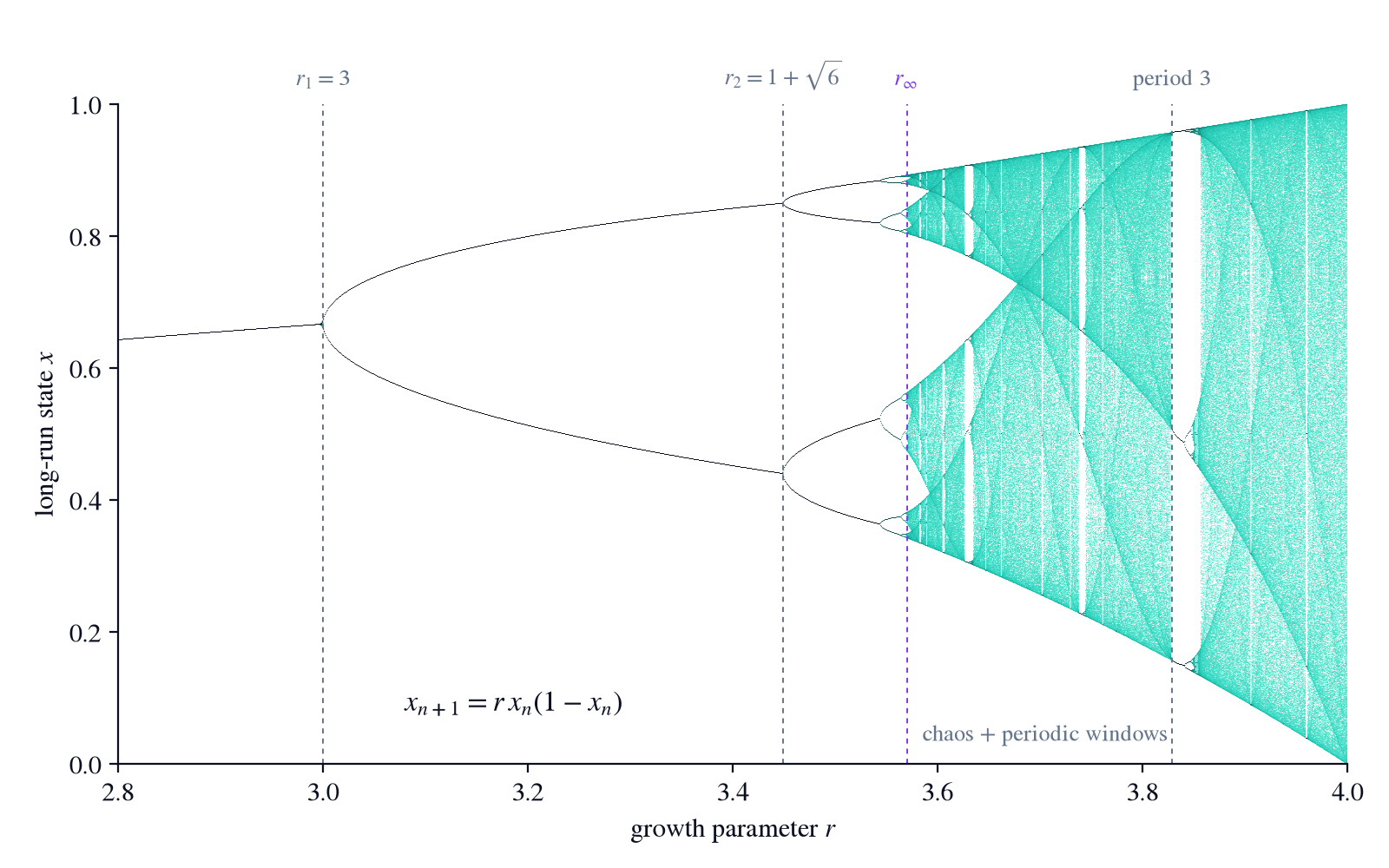
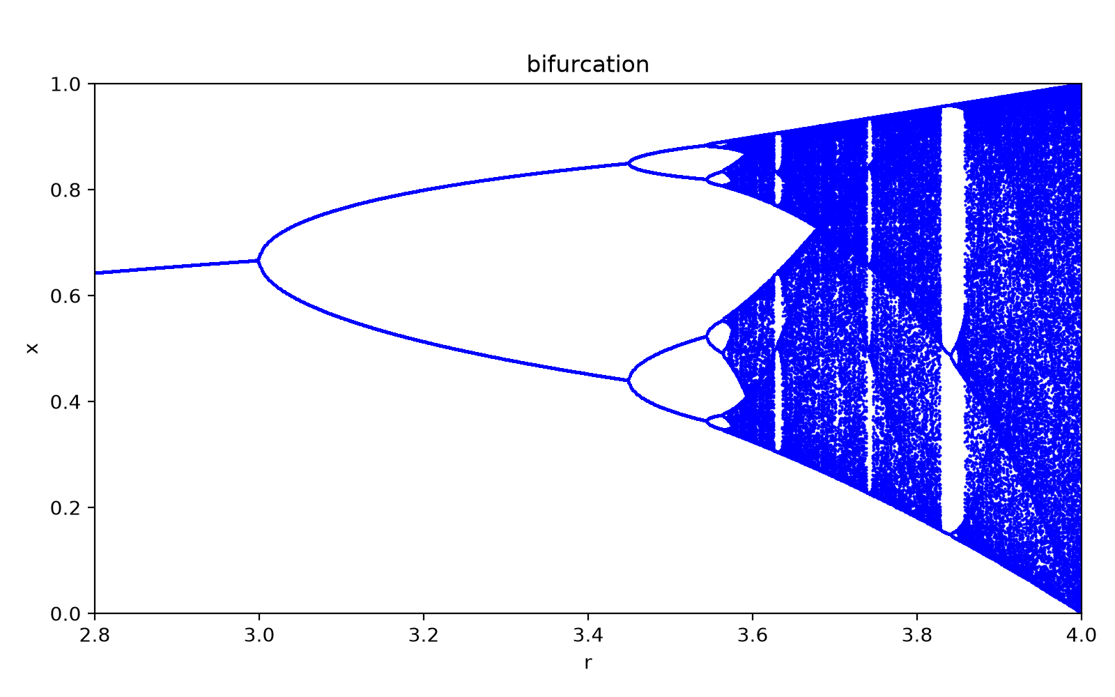
Drag the slider. On the left is the matplotlib default. On the right is the cleaned-up figure: density shading instead of a blue wall, labelled bifurcation points, real axis labels, journal typography.

Publication-ready bifurcation diagram of the logistic map with density shading and labelled bifurcation points. The same diagram with matplotlib defaults: solid blue points, generic title and bare axis labels. Before · defaults After
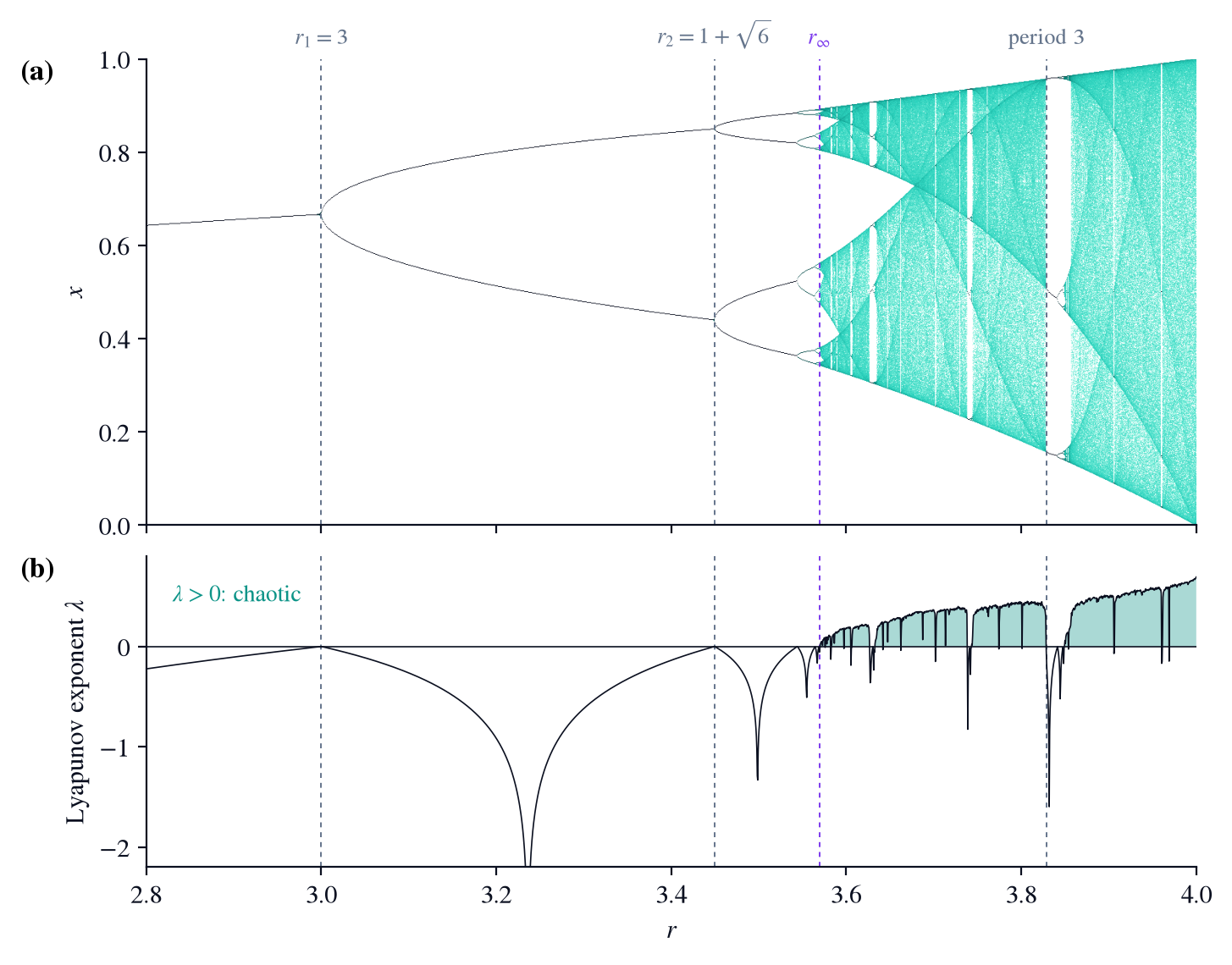
Two-panel figure: bifurcation diagram above, Lyapunov exponent below, sharing the r axis.
Figure 1. (a) Long-run states of the logistic map against r. (b) Lyapunov exponent λ on the same axis. Shading marks λ > 0. Dashed lines: r1 = 3, r2 = 1 + √6, the accumulation point r∞ ≈ 3.5699, and the opening of the period-3 window at 1 + √8. Periodic windows inside the chaotic band show up as dips below zero.
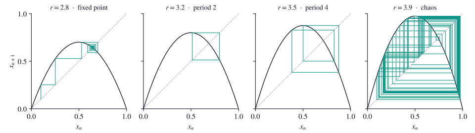
Four cobweb diagrams at r equal to 2.8, 3.2, 3.5 and 3.9, showing a fixed point, period 2, period 4 and chaos.
Figure 2. Cobweb diagrams for four values of r. At 2.8 the orbit spirals into a fixed point; at 3.2 and 3.5 it settles on cycles of period 2 and 4; at 3.9 it never repeats.

04 · Writing & polishing

Same content, tighter claims

You ask"Polish this paragraph for the introduction. Keep my meaning, make it precise."

You get the rewrite plus a short list of what changed and why, so you learn the pattern instead of just accepting edits.

Draft

In this work we study the logistic map which is a very famous and simple model that has very complicated dynamics. It is very well known that as the parameter r is increased the system goes through a series of period doublings and eventually becomes chaotic, this was shown by Feigenbaum. We compute the Feigenbaum constant numerically and we obtain a value which is very close to the known value of 4.669 which shows that our method works good.

Polished

We study the logistic map, xn+1 = r xn(1 − xn), a one-parameter model whose simple form hides notoriously rich dynamics (May, 1976). As r increases, the map undergoes a cascade of period-doubling bifurcations that accumulates at r∞ ≈ 3.5699, beyond which chaotic orbits appear. Feigenbaum (1978) showed that successive bifurcations close in geometrically, at a universal rate δ ≈ 4.6692. Locating the superstable parameters by Newton's method, we recover δ to seven significant figures.

What changed

  1. The equation appears on first mention, so the reader knows exactly which map.
  2. "Very famous … very complicated" becomes one precise claim with a citation.
  3. The comma splice is split, and "this was shown by Feigenbaum" now says what he showed.
  4. "Very close" becomes a number: seven significant figures.
  5. "Shows that our method works good" is gone. The agreement makes that point on its own.

Skills

The research pipeline

Each skill works on its own. Used together, they share one research/ folder instead of calling each other.

Paper Figures

Turn results into journal-ready scientific figures that never overstate the data: the right plot for the claim, a colour-blind-safe journal style, and a check before submission.

Test Readers

Find out how real readers will receive a draft before you send it: blind reader personas read it cold, a probe checks whether your message landed, and you get a severity-ranked report with a fix for every issue.

Citable Python Packages

Turn research scripts into a pip-installable, citable Python package: src/ layout with uv, ruff and pytest, CITATION.cff and a How to cite section, a lock file for reproducibility, and your code moved without rewrites.

Figure Editor

Turn the plots, micrographs and diagrams you already have into one labelled multi-panel figure at exact journal width, with placeholders for missing panels, a print-resolution check and a caption draft.

Figure Audit

Review your research figures before submission, or a manuscript's as a referee: what misleads, what slows the reader, what fails colour-blind and greyscale readers. Ranked findings with evidence, a minimal fix and a redesign, both redrawn.

Table Design

Turn a results CSV into the table your paper needs: booktabs LaTeX plus a Markdown copy for the README. Methods × datasets, mean ± SD rounded to match, best values in bold, missing runs marked and explained, rendered and checked.

Bifurcation Diagrams

Give your agent an ODE model and a parameter range; get a journal-ready bifurcation diagram computed from the equations: branches traced through folds, stability from the Jacobian, fold, branch and Hopf points located, every branch checked by simulation.

Claim Check

Before co-authors or reviewers see your draft, your agent checks every sentence about a result against the results file it cites: numbers within rounding, no verdict over an interval that includes zero, no hand conversions, one fact per citation.

Scientific Voice

Your agent tightens scientific prose in English and Spanish for submission: finding before caveat, one hedge sized to the evidence, no meta-commentary, verbs instead of buried nouns, false friends and mixed formats fixed. Numbers and terms never change.

Journal House Style

Name the journal, conference or thesis office, or hand over your own style sheet. Your agent builds a venue profile from its current guidelines, a source on every rule, then audits your draft against it and restructures and cuts it to fit.

Research Software

Your agent reviews the code behind your paper for leakage, unseeded randomness, floats compared without a tolerance and swallowed errors, fixes what it finds, pins your results with tests, and reruns everything until the same seed gives the same number.

Instructions Writer

Your agent rewrites a README, setup guide, reproduction steps or lab protocol from the facts in your project, then has a fresh agent follow it to the letter in a clean copy and fixes every step it had to guess.

Poster Layout

Turn your abstract, figures and data into a conference poster that reads from across the aisle: a title that states the result, one claim and one piece of evidence per zone, figures redrawn at printed size, and a checked one-page PDF at A0 or any size.

Q&A Prep

Your agent reads your own paper, slides or results, finds the weak spots a sharp questioner will hit, ranks the questions you'll get after a talk, poster or defence, and drafts short answers that stay inside what your material supports, with every number checked.

Talk Coach

Your agent transcribes your rehearsal on your own machine, measures where the minutes went, reads the talk as your audience will hear it, and gives you a cut list that fits your slot and three priorities with drills, every point tied to a timestamp and a quote.

Slide Architect

Turn your paper, figures and data into a research talk that lands: the finding by slide 3, a claim in every headline, figures redrawn for the screen, every number traced to your work, and an editable .pptx with speaker notes.

Modelling Paper

Your agent co-writes a modelling paper in any field: it pins the claim, writes the full Methods mathematics with a sourced notation table, checks the derivations against your code, never invents references, and keeps a rated list of reviewer objections.

How it works

Skills run inside the agent you already use

  1. 1

    Pick a skill

    Browse the skills on Agensi. Each listing says what it does and which tools it needs.

  2. 2

    Install it

    It loads into Claude Code, Cursor, Codex CLI and most other agents that read SKILL.md.

  3. 3

    Ask in plain words

    "Make this figure publication-ready." "Summarize the key papers on X." The skill handles the rest.